DAFT figure gallery

Figure 1.1Python

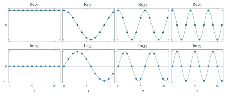
Characters of a cyclic group

Real and imaginary parts of the first four characters of \(\mathbb{Z}/12\mathbb{Z}\).

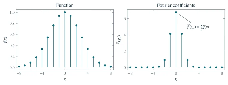
In the book p. 3 PDF Python source Run notebook Notebook

Figure 1.2Python

Fourier decomposition

An even bell-shaped function on \(\mathbb{Z}/17\mathbb{Z}\) and its real Fourier coefficients, with centered indices.

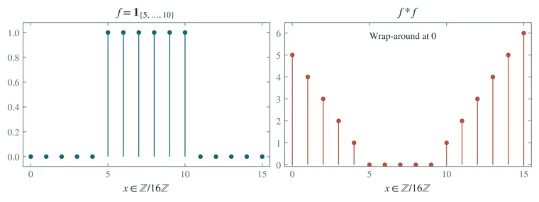
In the book p. 9 PDF Python source Run notebook Notebook

Figure 1.3Python

Circular convolution

Circular self-convolution of \(f=\mathbf{1}_{\{5,\ldots,10\}}\) on \(\mathbb{Z}/16\mathbb{Z}\). The maximum occurs at \(15\) modulo \(16\); the remaining values wrap around at \(0\).

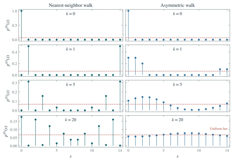
In the book p. 10 PDF Python source Run notebook Notebook

Figure 1.4Python

Random walks on a cyclic group

Random walks on \(\mathbb{Z}/15\mathbb{Z}\) with increment laws \((0,1/2,0,\ldots,0,1/2)\) and \((0.3,0.3,0.2,0,\ldots,0,0.1,0.1)\). Dashed lines show the uniform distribution.

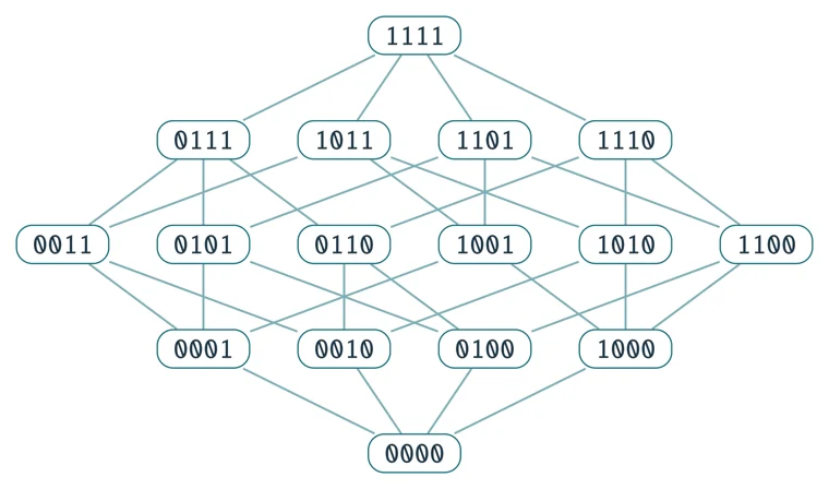
In the book p. 15 PDF Python source Run notebook Notebook

Figure 2.1TikZ

The Boolean cube

The Boolean cube \(\FF_2^4\), arranged by Hamming weight. Each edge changes exactly one coordinate.

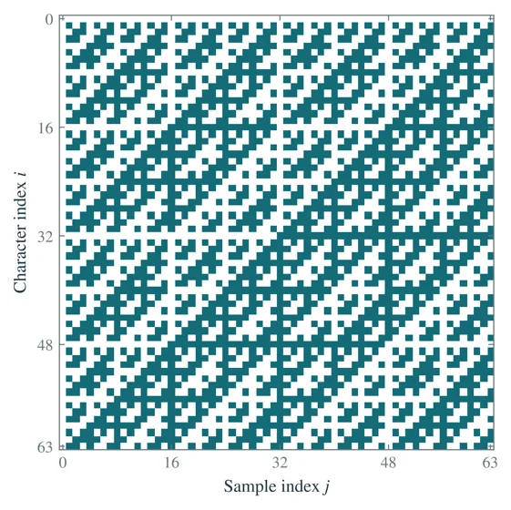
In the book p. 27 PDF Python source TikZ source

Figure 2.2Python

The Walsh matrix

The Walsh matrix \(W_{64}\) in natural order. White represents \(+1\) and dark teal represents \(-1\).

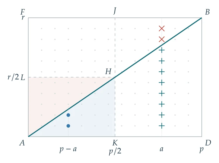
In the book p. 28 PDF Python source Run notebook Notebook

Figure 2.3TikZ

Quadratic reciprocity on a lattice

Lattice-point pairing in the geometric proof of quadratic reciprocity, illustrated with \(p=13\), \(r=11\), and \(a=10\).

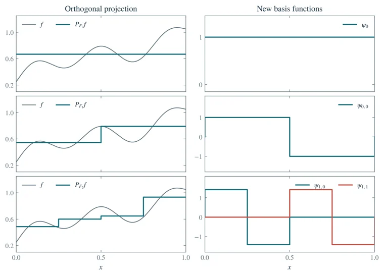
In the book p. 34 PDF Python source TikZ source

Figure 2.4Python

Successive Haar projections

Successive Haar projections onto \(F_0\), \(F_1\), and \(F_2\) (left), and the orthonormal basis functions added at each stage (right).

In the book p. 35 PDF Python source Run notebook Notebook

Figure 2.5TikZ

The Haar cascade

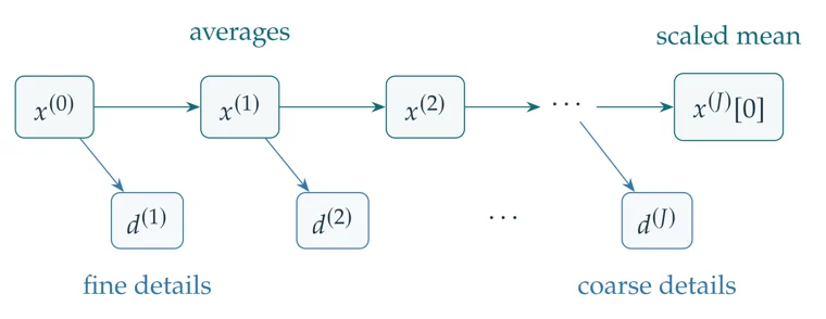
The Haar cascade: each stage separates scaling coefficients from details, which are stored from fine to coarse.

In the book p. 36 PDF Python source TikZ source

Figure 2.6Python

Discrete Haar transforms

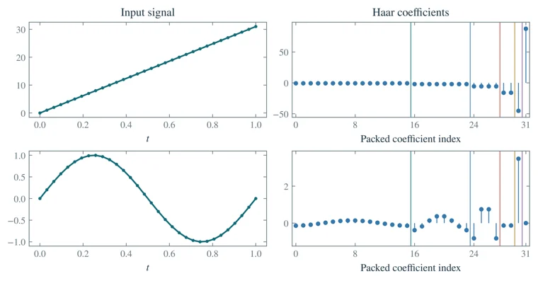
Two length-\(32\) signals and their orthonormal Haar coefficients. Colored separators mark the detail scales; the final coefficient is the scaled mean.

In the book p. 37 PDF Python source Run notebook Notebook

Figure 2.7Python

Natural and sequency order

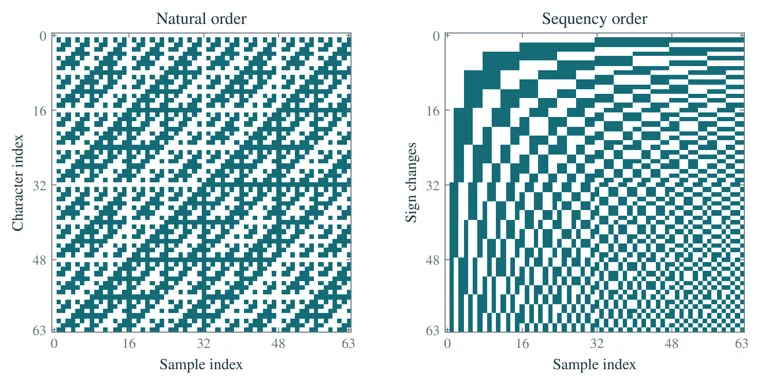
Walsh functions in natural order and in increasing sequency, with one basis function per row.

In the book p. 37 PDF Python source Run notebook Notebook

Figure 2.8Python

The Walsh spectrum

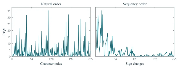
The Walsh spectrum of the oscillatory signal in Figure 2.9, in natural and sequency order.

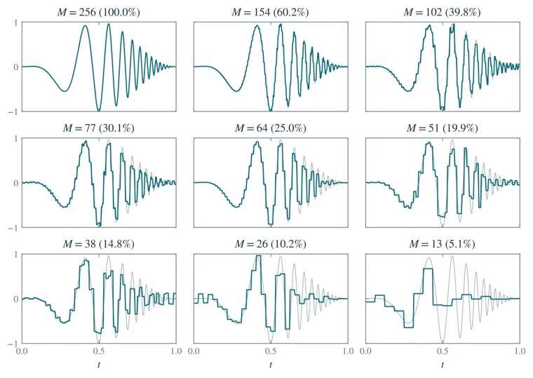
In the book p. 38 PDF Python source Run notebook Notebook

Figure 2.9Python

Walsh approximation of a signal

Progressive approximation of a signal by initial segments of the sequency-ordered Walsh basis. Each panel gives the exact retained coefficient count.

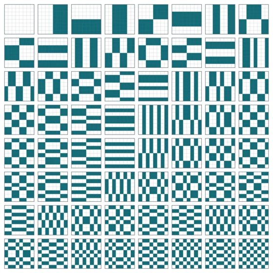
In the book p. 38 PDF Python source Run notebook Notebook

Figure 2.10Python

Two-dimensional Walsh functions

The \(64\) two-dimensional Walsh functions for \(8\times8\) images, ordered by total sequency and then vertical sequency, from left to right and top to bottom.

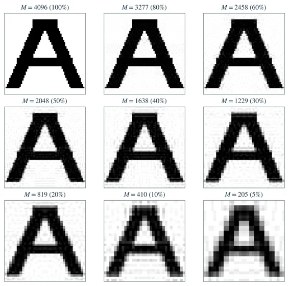
In the book p. 39 PDF Python source Run notebook Notebook

Figure 2.11Python

Walsh approximation of an image

Walsh approximations of a synthetic letter A, with exact retained coefficient counts. Every panel uses the same grayscale range.

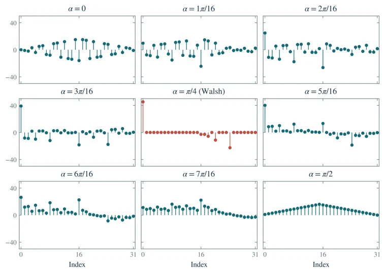
In the book p. 40 PDF Python source Run notebook Notebook

Figure 2.12Python

Intermediate Walsh transforms

Normalized tensor transforms \(2^{-n/2}A_\alpha^{\otimes n}\) of a triangular signal, with \(n=5\). The middle panel is the Walsh transform; the last reverses the input entries.

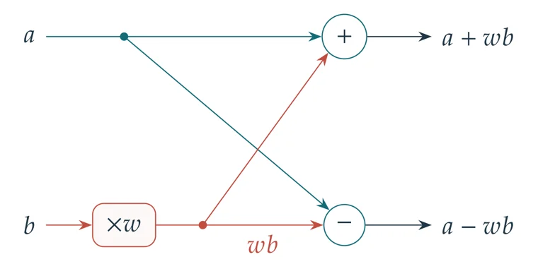
In the book p. 41 PDF Python source Run notebook Notebook

Figure 3.1TikZ

An FFT butterfly

An FFT butterfly: the same weighted value \(wb\) enters the sum and the difference, with \(w=\omega_N^{-k}\).

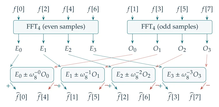
In the book p. 52 PDF Python source TikZ source

Figure 3.2TikZ

An eight-point FFT

The combination stage of an eight-point DIT FFT. Two four-point transforms produce \(E_k\) and \(O_k\); each butterfly combines \(E_k\) with \(\omega_8^{-k}O_k\).

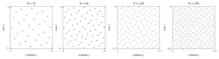
In the book p. 53 PDF Python source TikZ source

Figure 3.3Python

Bit-reversal matrices

Bit-reversal permutation matrices for \(N=32,64,128,256\). A dot in row \(i\) and column \(j\) means that the bits of \(j\) are those of \(i\) in reverse order.

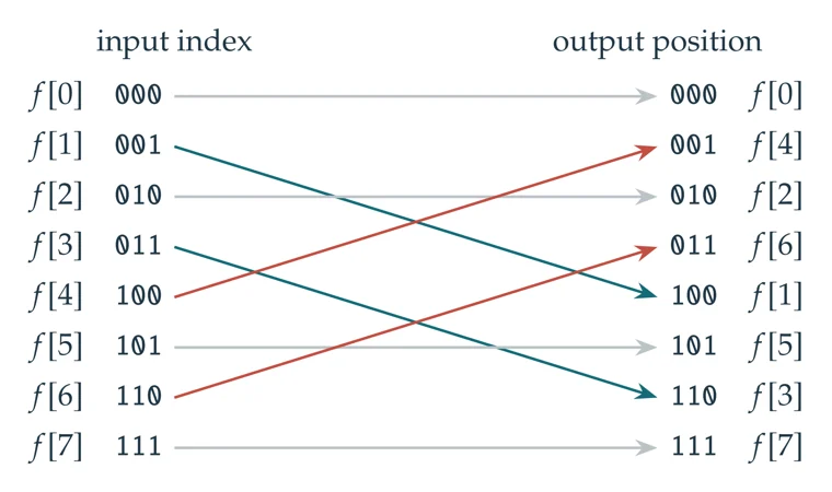
In the book p. 54 PDF Python source Run notebook Notebook

Figure 3.4TikZ

The bit-reversal permutation

Bit reversal on eight entries. The binary labels make the swaps \(1\leftrightarrow4\) and \(3\leftrightarrow6\) explicit; the other four indices are fixed.

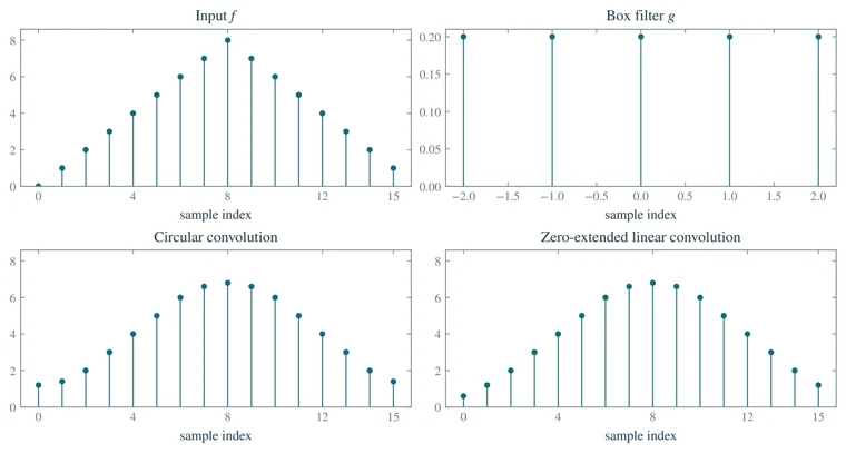
In the book p. 55 PDF Python source TikZ source

Figure 3.5Python

Linear and circular convolution

Circular and zero-extended linear convolution of a triangular signal with a unit-sum five-tap box filter. The outputs agree away from the endpoints.

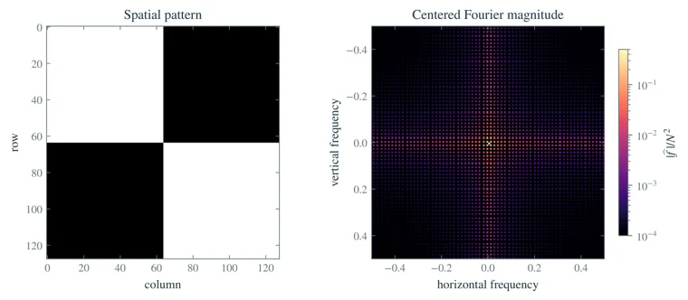
In the book p. 57 PDF Python source Run notebook Notebook

Figure 3.6Python

The two-dimensional DFT

A two-dimensional checker pattern and its centered Fourier magnitude. The logarithmic color scale reveals the weaker frequencies.

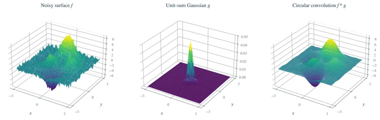
In the book p. 59 PDF Python source Run notebook Notebook

Figure 3.7Python

Two-dimensional convolution

Circular Gaussian smoothing of a noisy surface. The discrete kernel has unit sum; its center is shifted to index \((0,0)\) before the FFT.

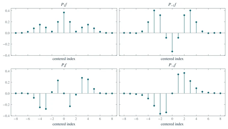
In the book p. 59 PDF Python source Run notebook Notebook

Figure 3.8Python

Fourier eigenspace projections

The four orthogonal components \(P_\lambda f\) of a real signal for the normalized DFT \(U\). Their sum is \(f\); even and odd components appear on separate rows.

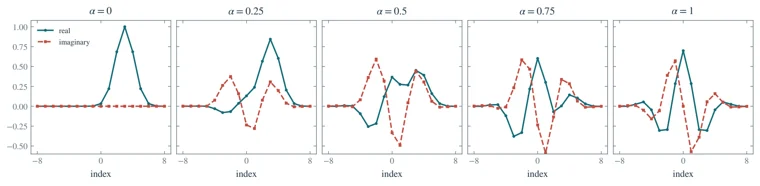
In the book p. 61 PDF Python source Run notebook Notebook

Figure 3.9Python

Intermediate Fourier transforms

The unitary transforms \(U^\alpha f\) for \(0\leq\alpha\leq1\), using the fixed phases in the text. Real and imaginary parts are shown separately.

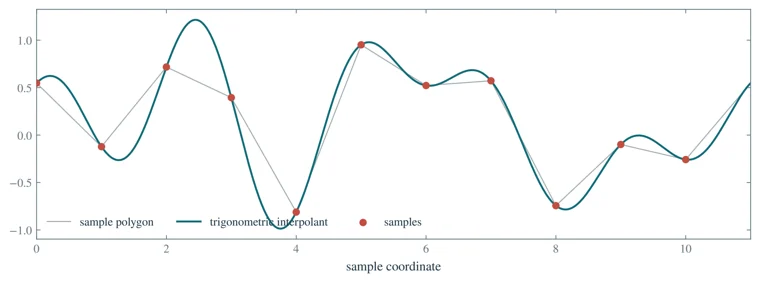
In the book p. 61 PDF Python source Run notebook Notebook

Figure 3.10Python

Trigonometric interpolation

Periodic trigonometric interpolation of eleven samples. The faint polygon joins the samples for reference; it is not an underlying continuous signal.

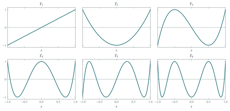
In the book p. 63 PDF Python source Run notebook Notebook

Figure 3.11Python

Chebyshev polynomials

The Chebyshev polynomials \(T_k(x)=\cos(k\arccos x)\) for \(k=1,\ldots,6\).

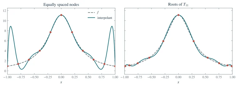
In the book p. 64 PDF Python source Run notebook Notebook

Figure 3.12Python

Choosing interpolation nodes

Degree-ten polynomial interpolation of \(f(x)=1/(0.3^2+x^2)\) at eleven equally spaced points and at the roots of \(T_{11}\). Both are Lagrange interpolants; the choice of nodes controls the endpoint oscillations.

In the book p. 65 PDF Python source Run notebook Notebook

Figure 3.13Python

Fractional differentiation

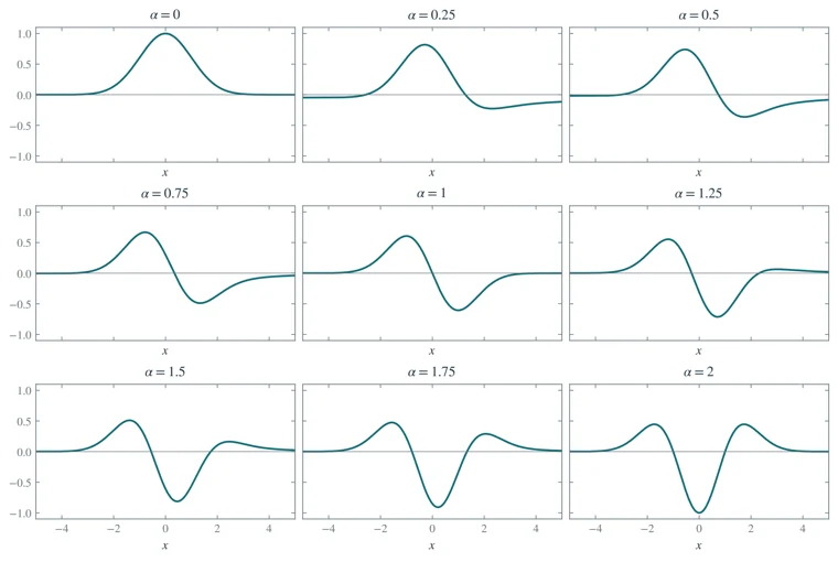
Fractional derivatives of \(e^{-x^2/2}\) for orders \(0\leq\alpha\leq2\), computed from the multiplier \((\imath\xi)^\alpha\) with the phase convention in the text.

In the book p. 66 PDF Python source Run notebook Notebook

Figure 3.14Python

Fractional Fourier matrices

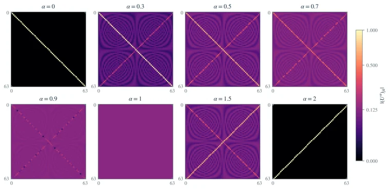
Entrywise magnitudes of the unitary matrices \(U^\alpha\), on one common nonlinear color scale. At \(\alpha=1\) every magnitude equals \(1/\sqrt N\); at \(\alpha=2\) the matrix is cyclic reversal.

In the book p. 66 PDF Python source Run notebook Notebook

Figure 3.15Python

Fractional transforms of a Gaussian

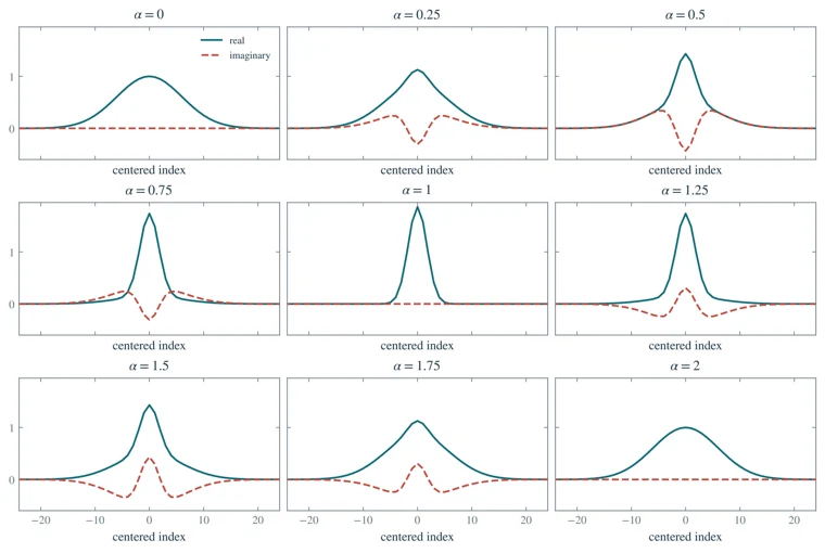
Unitary fractional Fourier transforms of a discrete Gaussian. The fixed eigenspace phases give a continuous family; at \(\alpha=2\) this even input is recovered.

In the book p. 67 PDF Python source Run notebook Notebook

Figure 3.16Python

Structured Fourier eigenvectors

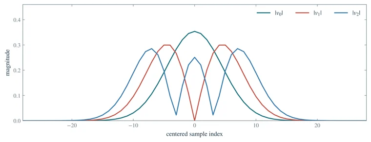
Magnitudes of the first three vectors in the structured DFT eigenbasis for \(N=128\), ordered by decreasing eigenvalue of \(S\). The index is centered for display.

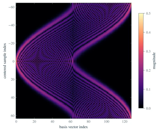
In the book p. 68 PDF Python source Run notebook Notebook

Figure 3.17Python

A Fourier eigenbasis

Magnitudes of the structured orthonormal eigenbasis for \(N=128\). Columns follow decreasing eigenvalues of \(S\), with even parity first in a tie; rows show centered sample indices.

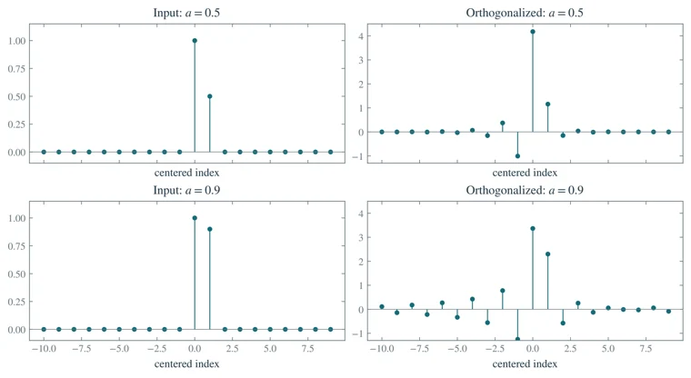
In the book p. 68 PDF Python source Run notebook Notebook

Figure 3.18Python

Orthogonalizing cyclic translates

Orthogonalizing the cyclic translates of \(f=\delta_0+a\delta_1\) on \(\mathbb{Z}/20\mathbb{Z}\), for \(a=0.5\) and \(a=0.9\). The output \(g\) satisfies \(|\widehat g|=\sqrt{20}\), as required by the normalized inner product.

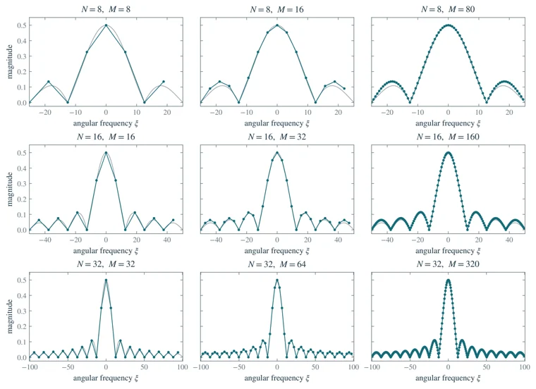
In the book p. 69 PDF Python source Run notebook Notebook

Figure 4.1Python

Sampling and zero padding

Sampling and zero padding for \(f=\mathbf1_{[1/2,1)}\). Rows change the number \(N\) of measured samples; columns change only the padded length \(M\). The DFT magnitudes include the quadrature factor \(1/N\); the faint curve is the continuous-transform magnitude.

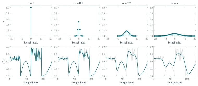
In the book p. 80 PDF Python source Run notebook Notebook

Figure 4.2Python

Gaussian smoothing of a signal

Gaussian kernels and their action on one fixed irregular signal. Widths are in sample units, and the signal is reflected at its endpoints. The first column is the exact identity kernel.

In the book p. 81 PDF Python source Run notebook Notebook

Figure 4.3Python

Impulse, frequency, and step responses

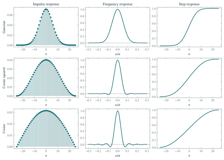
Impulse, frequency, and step responses of three unit-sum symmetric FIR kernels. The frequency plots show a neighborhood of zero; the step responses are cumulative sums of the impulse responses.

In the book p. 82 PDF Python source Run notebook Notebook

Figure 4.4Python

Gaussian smoothing of an image

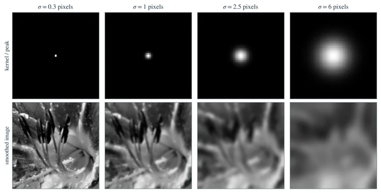
Discrete Gaussian kernels (top) and smoothing of the flower image (bottom), with reflected boundaries. Each kernel is displayed relative to its own peak; all image panels share the grayscale range \([0,1]\).

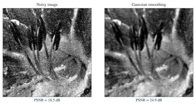
In the book p. 83 PDF Python source Run notebook Notebook

Figure 4.5Python

Image denoising

A flower image corrupted by additive Gaussian noise of standard deviation \(0.12\), and Gaussian smoothing with width \(0.9\) pixels. The displayed PSNR values use the same clean reference; intensity clipping is for display only.

In the book p. 83 PDF Python source Run notebook Notebook

Figure 4.6Python

Four regimes of polygon filtering

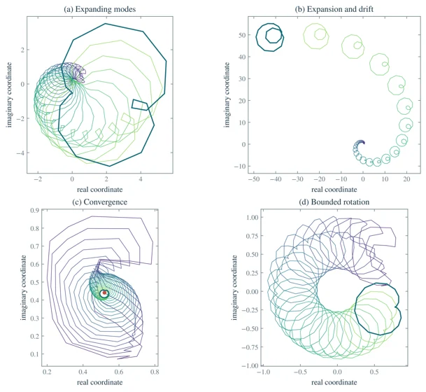
Four regimes of polygon filtering. Curves progress from the initial polygon to later iterates. Expanding active multipliers cause divergence; unit-modulus phases can keep the trajectory bounded without convergence.

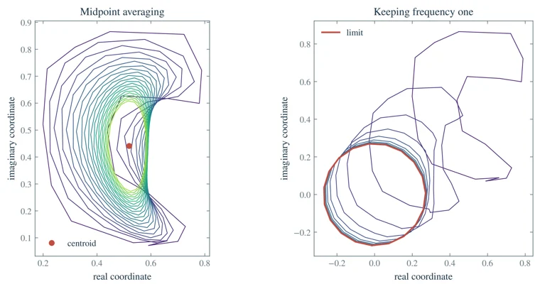
In the book p. 84 PDF Python source Run notebook Notebook

Figure 4.7Python

Filtering a polygon

Successive midpoint averaging converges to the vertex centroid (left). Keeping only frequency one produces a regular polygon of radius \(|\widehat\Pi[1]|/N\) (right). Red marks indicate the limits.

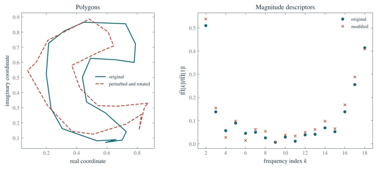
In the book p. 85 PDF Python source Run notebook Notebook

Figure 4.8Python

Fourier shape descriptors

A polygon and a perturbed, rotated version, with their magnitude-based Fourier descriptors. The perturbation changes the descriptor; the rotation alone would leave it unchanged.

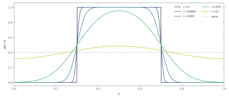
In the book p. 86 PDF Python source Run notebook Notebook

Figure 4.9Python

The spectral heat equation

Spectral heat evolution of an interval indicator on the unit circle, with conductivity \(\kappa=1/2\). The mean is preserved and the nonconstant Fourier modes decay.

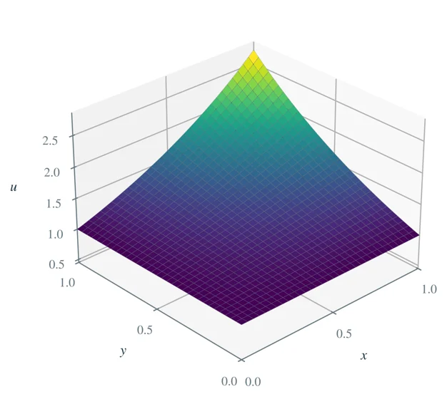
In the book p. 88 PDF Python source Run notebook Notebook

Figure 4.10Python

Solving the Poisson equation

Dirichlet Poisson solution with reference \(u(x,y)=e^{xy}\), on a grid with \(N=32\) intervals per axis.

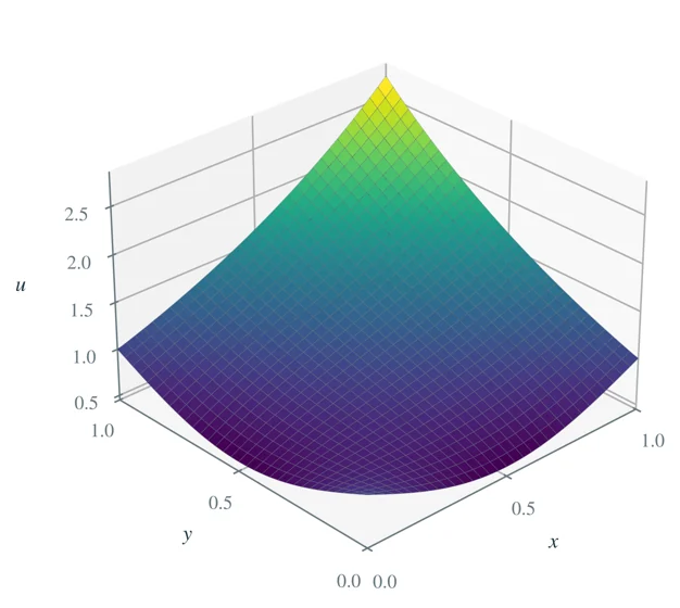
In the book p. 89 PDF Python source Run notebook Notebook

Figure 4.11Python

Changing the boundary values

Dirichlet Poisson solution with reference \(u(x,y)=e^{xy}\), on a grid with \(N=32\) intervals per axis.

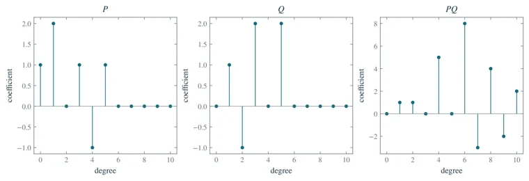
In the book p. 89 PDF Python source Run notebook Notebook

Figure 4.12Python

Multiplying polynomials by convolution

Coefficient vectors of \(P\), \(Q\), and their product. Length-eleven FFT convolution agrees with the ordinary degree-ten polynomial product.

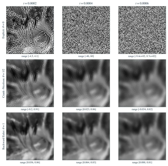
In the book p. 90 PDF Python source Run notebook Notebook

Figure 4.13Python

Time stepping for the heat equation

Three time steps for the same flower image, with \(N=128\) and \(h=0.0002\). Explicit Euler is unstable; Crank–Nicolson is stable but weakly damps high frequencies; backward Euler damps them strongly. All images use \([0,1]\), and each panel reports its actual value range.

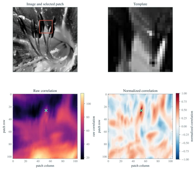
In the book p. 92 PDF Python source Run notebook Notebook

Figure 4.14Python

Template matching by correlation

Template matching in the flower image. The red box identifies the extracted patch; crosses mark its location in the raw and normalized correlation maps. Only complete-template positions are included.

In the book p. 94 PDF Python source Run notebook Notebook

Figure 4.15Python

Rotating an image with Fourier shears

Rotations of the flower image by three Fourier shears. The odd grid avoids a Nyquist ambiguity; a white margin limits wraparound. Cropping and intensity clipping are applied only to the displayed results.

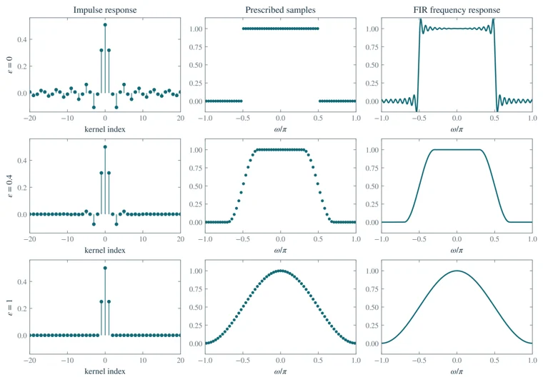
In the book p. 95 PDF Python source Run notebook Notebook

Figure 4.16Python

Designing low-pass filters

Low-pass filters with increasingly wide raised-cosine transitions. The columns show the centered impulse response, the prescribed DFT samples, and the densely sampled FIR frequency response.

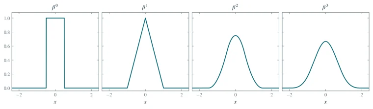
In the book p. 96 PDF Python source Run notebook Notebook

Figure 4.17Python

Centered B-splines

Centered B-splines of degrees zero through three. Their support is \([-(n+1)/2,(n+1)/2]\).

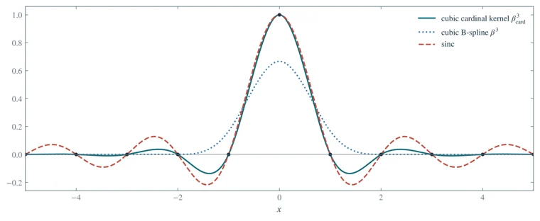
In the book p. 97 PDF Python source Run notebook Notebook

Figure 4.18Python

Cardinal splines and sinc

The cubic cardinal kernel, the cubic B-spline, and sinc. The cardinal kernel and sinc equal one at zero and vanish at every other integer; the cubic B-spline requires a prefilter.

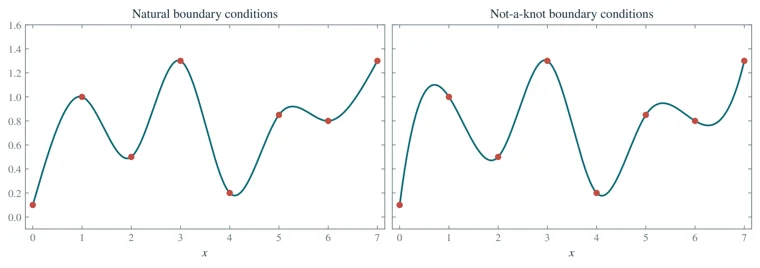
In the book p. 97 PDF Python source Run notebook Notebook

Figure 4.19Python

Boundary conditions for cubic splines

Cubic interpolation of the same eight samples with natural and not-a-knot boundary conditions. Natural conditions set the endpoint second derivatives to zero.

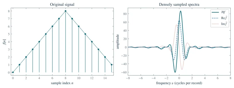
In the book p. 98 PDF Python source Run notebook Notebook

Figure 5.1Python

Hartley and Fourier spectra

A triangular signal and its densely evaluated Fourier and Hartley spectra. The Hartley spectrum equals the real part minus the imaginary part of the DFT. Zero padding changes only the frequency grid.

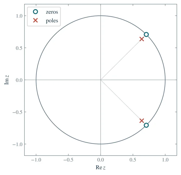
In the book p. 111 PDF Python source Run notebook Notebook

Figure 5.2Python

Poles and zeros of a notch filter

Zeros on the unit circle and poles at radius \(0.9\) for a notch filter at angular frequencies \(\pm\pi/4\). Circles mark zeros; crosses mark poles.

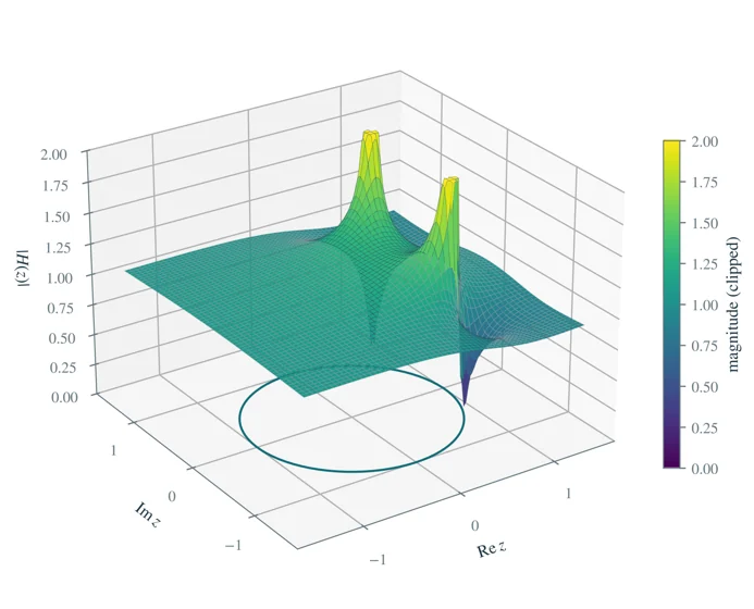
In the book p. 113 PDF Python source Run notebook Notebook

Figure 5.3Python

The notch-filter transfer function

Magnitude of the rational notch-filter transfer function in the complex plane. Values above two are clipped to reveal the zeros and pole neighborhoods. The causal Laurent series converges for \(|z|>0.9\).

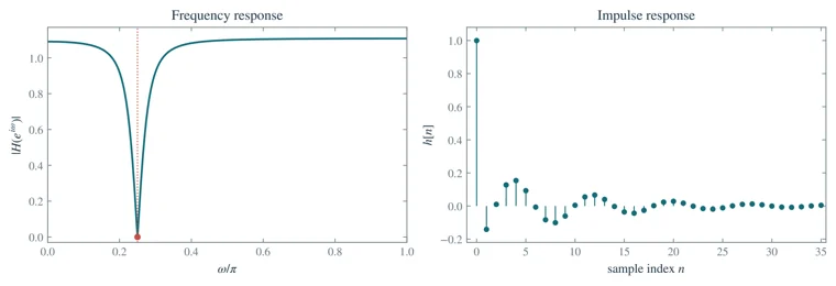
In the book p. 114 PDF Python source Run notebook Notebook

Figure 5.4Python

Notch-filter responses

Frequency-response magnitude and causal impulse response of the notch filter. The response vanishes at angular frequency \(\pi/4\).

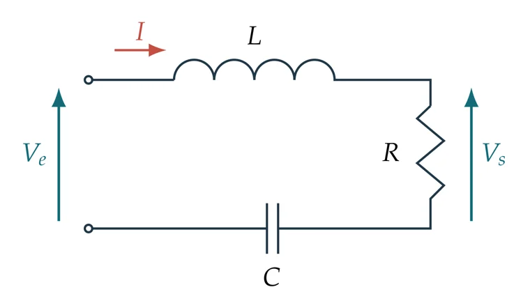
In the book p. 114 PDF Python source Run notebook Notebook

Figure 5.5TikZ

A series RLC circuit

A series RLC circuit, with the output voltage \(V_s\) measured across the resistor and the input \(V_e\) across the two left terminals.

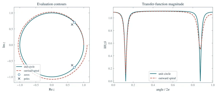
In the book p. 115 PDF Python source TikZ source

Figure 5.6Python

Contours for the z-transform

The notch-filter transfer function evaluated on a unit circle and an outward logarithmic spiral. Both contours lie in the causal region of convergence; leaving the unit circle changes the depth of the notches.

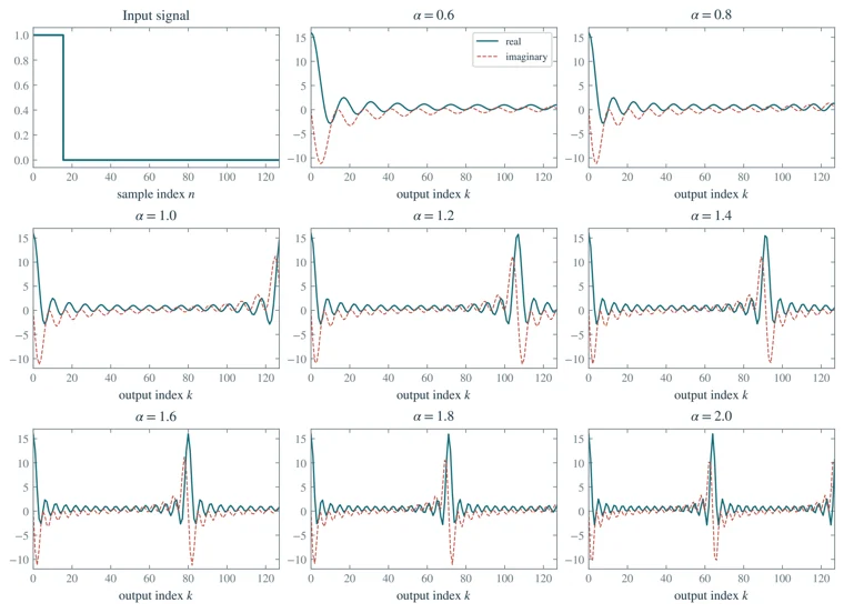
In the book p. 116 PDF Python source Run notebook Notebook

Figure 5.7Python

Scaled-frequency Fourier transforms

Scaled-frequency Fourier transforms of an interval indicator. The real and imaginary parts share the same scale. Changing \(\alpha\) changes the sampled frequency grid.

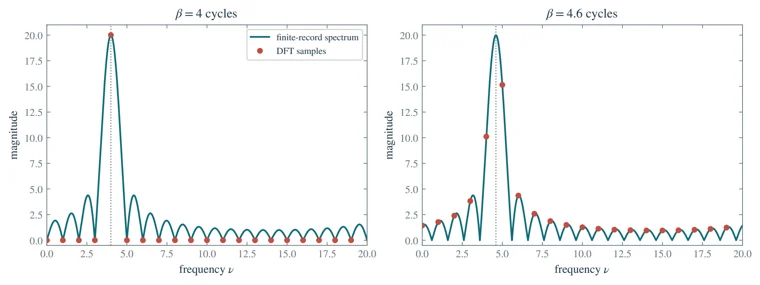
In the book p. 118 PDF Python source Run notebook Notebook

Figure 5.8Python

Spectral leakage

Finite-record spectra of sinusoids with integer and noninteger numbers of cycles. The continuous curves evaluate the finite sum; the dots are DFT samples. The vertical line marks the generating frequency.

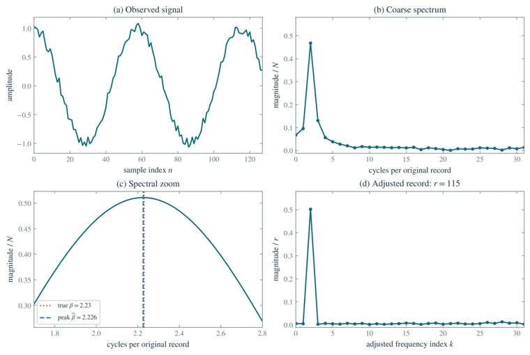
In the book p. 118 PDF Python source Run notebook Notebook

Figure 5.9Python

Zooming into a spectrum

A noisy cosine, its coarse spectrum, a local spectral zoom, and an adjusted spectrum after shortening the record using the estimated peak. Spectral magnitudes are divided by the respective record lengths. The generating frequency is distinguished from its estimate.

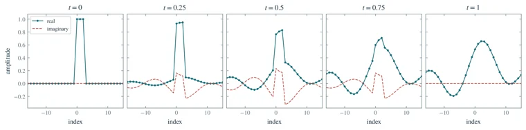
In the book p. 119 PDF Python source Run notebook Notebook

Figure 5.10Python

Fractional Hartley transforms

Real and imaginary parts of fixed-branch unitary Hartley powers \(V^t f\), with \(V=\mathcal{H}/\sqrt N\). All panels use the same amplitude scale and preserve the norm.

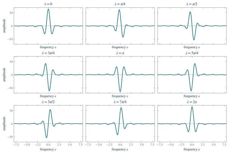
In the book p. 120 PDF Python source Run notebook Notebook

Figure 5.11Python

Generalized Hartley transforms

Generalized Hartley transforms of the same triangular signal. The phase \(\lambda\) changes the relative cosine and sine contributions; the two endpoint panels illustrate the \(2\pi\) periodicity.

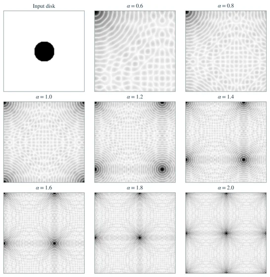
In the book p. 121 PDF Python source Run notebook Notebook

Figure 5.12Python

Scaled-frequency image transforms

Magnitudes of scaled-frequency two-dimensional Fourier transforms of a disk. Spectral panels share the contrast mapping \(\log(1+100|G_2|/\sum f)/\log(101)\), shown dark on white; the input panel uses ordinary grayscale.

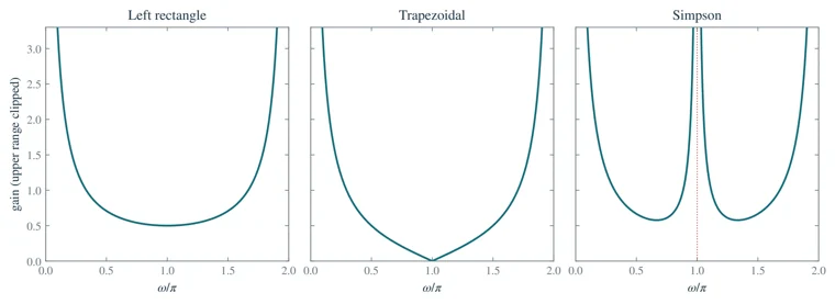
In the book p. 123 PDF Python source Run notebook Notebook

Figure 5.13Python

Quadrature filter responses

Magnitudes of the rectangle, trapezoidal, and Simpson integration filters for \(\Delta=1\). The poles at zero frequency and the additional Simpson pole at the Nyquist frequency are excluded from the plotted grid.

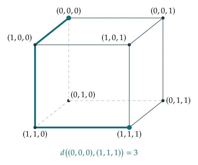
In the book p. 127 PDF Python source Run notebook Notebook

Figure 6.1TikZ

Hamming distance on the cube

Hamming distance on \(\FF_2^3\). Each cube edge changes one coordinate; the highlighted shortest path has three edges.

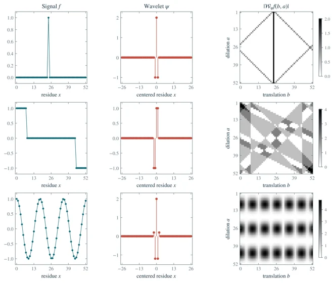
In the book p. 136 PDF Python source TikZ source

Figure 7.1Python

Wavelets over a finite field

Wavelets on \(\FF_{53}\): the signal, the centered wavelet, and the magnitude of its affine-group transform. Translation \(b\) is horizontal and nonzero dilation \(a\) is vertical. Each row has its own indicated magnitude scale. The first signal has nonzero mean, which the mean-zero wavelet removes.

In the book p. 169 PDF Python source Run notebook Notebook